Tutorial: Build a Rhino application using shiny.fluent

Hello World with rhino and shiny.fluent

Getting started with our development environment

Let us first install and create our rhino project structure. Note: Ensure Rhino v1.4.0 or later is installed for this tutorial.

To install rhino, please run the following in the R console:

# In R console
install.packages("rhino")

Now, initialize a new rhino application. You can do it either by using RStudio Wizard or a function rhino::init().

More details on how to create a Rhino app can be found in the Rhino tutorial.

You will notice that the working directory now has a proper folder structure along with some other files.

Rhino relies on the renv package for dependency management. To add the shiny.fluent package to our project, first, we need to install it.

Additionally, we will be also using the dplyr, ggplot2, plotly and tibble package for this application. To save us time in the tutorial we will install them all here. Please note that for every new package you add, you will need to install them, add them to dependencies.R, and run renv::snapshot() to update the renv.lock file.

# In R console
renv::install(c("dplyr", "ggplot2", "plotly", "shiny.fluent", "tibble"))

Now that the packages are installed, head over to the dependencies.R file and add shiny.fluent to it along with the others as shown below.

# dependencies.R

# This file allows packrat (used by rsconnect during deployment) to pick up dependencies.
library(dplyr)
library(ggplot2)
library(plotly)
library(rhino)
library(shiny.fluent)
library(tibble)

Upon saving the modified file, please take a snapshot of the dependencies so that the renv.lock file is updated.

# In R console
renv::snaphot()

If you now check the renv.lock file, you will see it is updated with the shiny.fluent and other packages.

Our first development on the app

Upon viewing the default app/main.R file, you will notice that the code does not have any usage of shiny.fluent package to generate the UI. So, let us introduce shiny.fluent and use it in our code to generate some text!

# app/main.R

box::use(
  shiny[moduleServer, NS],
  shiny.fluent[fluentPage, Text],
)

#' @export
ui <- function(id) {
  ns <- NS(id)
  fluentPage(
    Text("Sales Data Dashboard", variant = "xxLarge")
  )
}

#' @export
server <- function(id) {
  moduleServer(id, function(input, output, session) {

  })
}

The above code uses fluentPage and Text from shiny.fluent package to render the UI and the sentence - “Sales Data Dashboard”. You will also notice the NS(id) used in the code to return a namespace function, which has been saved as ns and will be invoked later in the shiny module.

Now when you run the app, you should be seeing this -

Note: If you check the built-in testcases once changes are introduced, running rhino::test_r() will give you errors. To avoid failed GitHub Actions for now (in case you are pushing your code to GitHub), you may empty the test cases present in tests/testthat/test-main.R.

Show Data in a Table via a rhino module

So, in this section, we will introduce a table to our application that displays random imaginary sales deals. The dataset comes from the shiny.fluent package itself - fluentSalesDeals.

Creating the module

In the app/view/ folder, let us create a new file and name it datatable.R

This app/view/datatable.R file will be used to display the data table on the UI and we will call this module in the app/main.R file once done. Here is the code

# app/view/datatable.R

box::use(
  shiny[div, moduleServer, NS, renderUI, uiOutput],
  shiny.fluent[DetailsList, Text, fluentSalesDeals],
)

#' @export
ui <- function(id) {
  ns <- NS(id)
    div(
      Text("A randomly generated dataset of imaginary sales deals", variant = "large"),
      uiOutput(ns("datatable"))
    )
}

#' @export
server <- function(id) {
  moduleServer(id, function(input, output, session) {
    output$datatable <- renderUI({
      DetailsList(items = fluentSalesDeals)
    })
  })
}

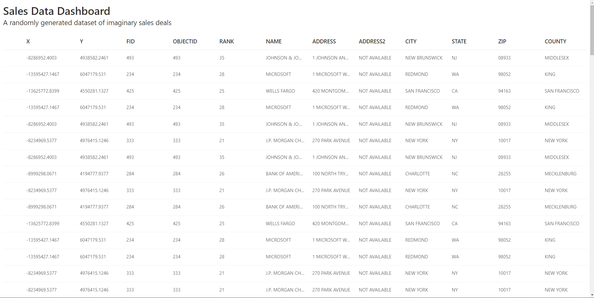
fluentSalesDeals is a dataset available with the shiny.fluent package.

So, here we are using DetailsList function in the server side to render the table on the UI.

Calling the module

Our shiny module app/view/datatable.R is ready, but unless we call it in the app/main.R file, we won’t see any changes on the app. Let us thus go to app/main.R file and edit it with the following code -

# app/main.R

box::use(
  shiny[moduleServer, NS],
  shiny.fluent[fluentPage, Text],
)

box::use(
  app/view/datatable,
)

#' @export
ui <- function(id) {
  ns <- NS(id)
  fluentPage(
    Text("Sales Data Dashboard", variant = "xxLarge"),
    datatable$ui(ns("datatable"))
  )
}

#' @export
server <- function(id) {
  moduleServer(id, function(input, output, session) {
    datatable$server("datatable")
  })
}

This code in the app/main.R file is based the concept of Shiny modules where box modules in rhino are used.

Notice here that we have called the datatable module by importing it to our main application file first. It is now, that the main module will be able to use exported functions from app/view/datatable.R module.

Now run the app. You should be seeing something like this -

Show informative columns with meaningful names

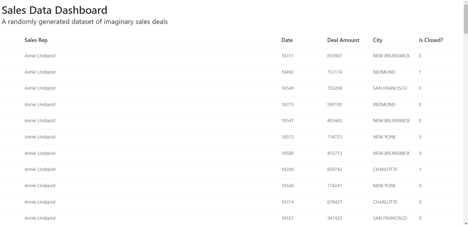
We will no more display all the columns that come with the dataset. Instead, we will display the "rep_name", "date", "deal_amount", "city", "is_closed" columns.

But for that we need to make the names more readable. So, we will assign proper names for every fields using the tibble package.

columns <- tibble(
  fieldName = c("rep_name", "date", "deal_amount", "city", "is_closed"),
  name = c("Sales Rep", "Date", "Deal Amount", "City", "Is Closed?")
)

Also, we need to mention in the DetailsList() function to only display the names we just assigned in the columns object. Here is how the code gets modified -

# app/view/datatable.R

box::use(
  shiny[div, moduleServer, NS, renderUI, uiOutput],
  shiny.fluent[DetailsList, Text, fluentSalesDeals],
  tibble[tibble],
)

columns <- tibble(
  fieldName = c("rep_name", "date", "deal_amount", "city", "is_closed"),
  name = c("Sales Rep", "Date", "Deal Amount", "City", "Is Closed?")
)

#' @export
ui <- function(id) {
  ns <- NS(id)
  div(
    Text("A randomly generated dataset of imaginary sales deals", variant = "large"),
    uiOutput(ns("datatable"))
  )
}

#' @export
server <- function(id) {
  moduleServer(id, function(input, output, session) {
    output$datatable <- renderUI({
      # This issue should be solved in the next `box` release.
      DetailsList(items = fluentSalesDeals, columns = columns)
    })
  })
}

Remember to include tibble inside box::use(), else the code will not be able to use the package. Upon running the app with all these changes, you should see the improved table -

Add a simple toggle input feature for the table with basic styling

Till now, we could only view table with all the data it has. We will now add a functionality to view those rows in the table where value of the “Is Closed?” column is 1 by default and provide a toggle to the user to also include results where the value is 0. The “Is Closed?” column basically indicates whether the deal is closed or not with values 0 and 1 where 0 means False/No and 1 means True/Yes.

We will make use of the dplyr package now. We will use Toggle.shinyInput from shiny.fluent package which represents a physical switch that allows someone to choose between two mutually exclusive options. For example,“On/Off”,“Show/Hide”. Choosing an option should produce an immediate result.

In the UI, we include the code for showing the toggle for input - Toggle.shinyInput(ns("includeOpen"), label = "Include open deals"), and work on the input provided inside the server section

So, the app/view/datatable.R file now is modified to -

# app/view/datatable.R

box::use(
  dplyr[filter],
  shiny[div, moduleServer, NS, reactive, renderUI, uiOutput],
  shiny.fluent[DetailsList, Text, Toggle.shinyInput, fluentSalesDeals],
  tibble[tibble],
)

columns <- tibble(
  fieldName = c("rep_name", "date", "deal_amount", "city", "is_closed"),
  name = c("Sales Rep", "Date", "Deal Amount", "City", "Is Closed?")
)

#' @export
ui <- function(id) {
  ns <- NS(id)
  div(
    Text("A randomly generated dataset of imaginary sales deals", variant = "large"),
    div(
      class = "ms-depth-4",
      Toggle.shinyInput(ns("includeOpen"), label = "Include open deals")
    ),
    uiOutput(ns("datatable")),
  )
}

#' @export
server <- function(id) {
  moduleServer(id, function(input, output, session) {
    filtered_deals <- reactive({
      fluentSalesDeals |> filter(
        is_closed | input$includeOpen
      )
    })
    output$datatable <- renderUI({
      DetailsList(items = filtered_deals(), columns = columns)
    })
  })
}

This code is being used to determine whether open deals (i.e. deals that have not been closed) should be included in the filtered data or not. The | symbol between the two conditions is the logical OR operator, which means that the filter() function will return all rows where either is_closed is TRUE or input$includeOpen is TRUE.

Also, please notice that we have added an additional style to the class ms-depth-4 in the app/style/main.scss file. ms-depth-X classes are a part of Microsoft’s Fluent UI and provide elevation (depth) to components.

Here is the app/style/main.scss file now -

// app/style/main.scss

.ms-depth-4 {
    display: flex;
    flex-wrap: wrap;
    padding: 5px;
}

If you try running the application right now, you will not see any changes. That is because rhino uses minified app/static/app.min.css for styling. To use it, you will need to build it using the rhino function -

# in R console
rhino::build_sass()

Please refer to rhino documentation for more details on styling.

So, this is how the app looks and works now!

Improve visuals and layout for the table with elevated cards

We can create cards with elevations just like in Fluent UI documentation, as we partially covered it above. For creating cards, we can use Stack from shiny.fluent.

We will also style the data table area. The following code does the following -

• Confines the height and width of the table area.
• Creates an elevated card around the data table area.

# app/view/datatable.R

box::use(
  dplyr[filter],
  shiny[div, moduleServer, NS, reactive, renderUI, span, uiOutput],
  shiny.fluent[DetailsList, Stack, Text, Toggle.shinyInput, fluentSalesDeals],
  tibble[tibble],
)

columns <- tibble(
  fieldName = c("rep_name", "date", "deal_amount", "city", "is_closed"),
  name = c("Sales Rep", "Date", "Deal Amount", "City", "Is Closed?")
)

#' @export
ui <- function(id) {
  ns <- NS(id)
  div(
    Text("A randomly generated dataset of imaginary sales deals", variant = "large"),
    div(
      class = "ms-depth-4",
      Toggle.shinyInput(ns("includeOpen"), label = "Include open deals")
    ),
    Stack(
      horizontal = TRUE,
      tokens = list(padding = 20, childrenGap = 10),
      span(class = "ms-depth-8", uiOutput(ns("datatable")))
    )
  )
}

#' @export
server <- function(id) {
  moduleServer(id, function(input, output, session) {
    filtered_deals <- reactive({
      fluentSalesDeals |> filter(
        is_closed | input$includeOpen
      )
    })
    output$datatable <- renderUI({
      DetailsList(items = filtered_deals(), columns = columns)
    })
  })
}

The Stack element in the code allows for stacking multiple elements vertically or horizontally.

The horizontal argument is set to TRUE to horizontally stack the two elements. The tokens argument is a list that specifies the padding and the gap between the two elements. In this case, the padding is set to 20 and the childrenGap is set to 10. This will add a padding of 20 pixels and a gap of 10 pixels between the other span of the Stack element.

The span element has a class attribute set to ms-depth-8. This is a class provided by the Microsoft fluent UI that adds a shadow effect to the element, giving it a depth effect. The uiOutput element is used to render the DetailsList element that contains the filtered data.

The additional style for the class ms-depth-8 is added in the app/style/main.scss file. So it now is modified to -

// app/style/main.scss

.ms-depth-4 {
    display: flex;
    flex-wrap: wrap;
    padding: 5px;
}

.ms-depth-8 {
    height: 500px;
    overflow: overlay;
    width: 50%;
    display: inline-block;
}

The Sass code limits the height of the table to 500 pixels, width to 50% of the screen size and allows scrolling through the data. Similar to the previous usecase, we would again have to repeat the Sass building process with rhino as the file has been updated.

# in R console
rhino::build_sass()

So, this is how the UI should look now -

Note that we now we have space beside the table for additional UI component(s).

Create separate rhino modules for toggle input and datatable

Now that we have successfully introduced a datatable and a toggle input in our application, let us further create different Rhino modules for them!

We already have the datatable module with us. We will thus create one more module - app/view/toggle.R and make some modifications in app/view/datatable.

These modules will be called from the main file.

The app/view/toggle.R module

# app/view/toggle.R

box::use(
  dplyr[filter],
  shiny[div, moduleServer, NS, reactive],
  shiny.fluent[Text, Toggle.shinyInput, fluentSalesDeals],
)

#' @export
ui <- function(id) {
  ns <- NS(id)
  div(
    class = "ms-depth-4",
    Toggle.shinyInput(ns("includeOpen"), label = "Include open deals")
  )
}

#' @export
server <- function(id) {
  moduleServer(id, function(input, output, session) {
    filtered_deals <- reactive({
      fluentSalesDeals |> filter(
        is_closed | input$includeOpen
      )
    })
    return(filtered_deals)
  })
}

This module displays a toggle input item on the UI which the user can interact with. The styling remains the same as we discussed in the previous sections.

As the user interacts with the toggle input, the data is filtered in the server. This filtered data is returned to the main module.

The modified app/view/datatable.R module

As the toggle module returns the filtered data, it is used in the datatable module so that the data is displayed on a table accordingly. Hence, our datatable module is modified as shown below -

# app/view/datatable.R

box::use(
  shiny[moduleServer, NS, reactive, renderUI, uiOutput],
  shiny.fluent[DetailsList],
  tibble[tibble],
)

columns <- tibble(
  fieldName = c("rep_name", "date", "deal_amount", "city", "is_closed"),
  name = c("Sales Rep", "Date", "Deal Amount", "City", "Is Closed?")
)

#' @export
ui <- function(id) {
  ns <- NS(id)
  uiOutput(ns("datatable"))
}

#' @export
server <- function(id, data) {
  moduleServer(id, function(input, output, session) {
    output$datatable <- renderUI({
      DetailsList(items = data(), columns = columns)
    })
  })
}

Please notice, that inside the server function, the response obtained from the toggle module earlier is also passed on to be used in displaying the data in a table.

We are not returning any information from this module to the main module as it’s sole purpose is to display given data in a table with desired columns in an easily readable form.

The modified app/main.R module

Since we modified the modules, app/main.R also has to be modified.

# app/main.R

box::use(
  shiny[moduleServer, NS, span],
  shiny.fluent[fluentPage, Stack, Text],
)

box::use(
  app/view/datatable,
  app/view/toggle,
)

#' @export
ui <- function(id) {
  ns <- NS(id)
  fluentPage(
    Text("Sales Data Dashboard", variant = "xxLarge"),
    Text("A randomly generated dataset of imaginary sales deals", variant = "large"),
    toggle$ui(ns("toggle")),
    Stack(
      horizontal = TRUE,
      tokens = list(padding = 20, childrenGap = 10),
      span(class = "ms-depth-8", datatable$ui(ns("datatable")))
    )
  )
}

#' @export
server <- function(id) {
  moduleServer(id, function(input, output, session) {
    data <-toggle$server("toggle")
    datatable$server("datatable", data)
  })
}

Here we have used the toggle and datatable modules and called them from the code.

Create a rhino module to render a bar chart with logic in a helper function

We will now add a bar chart that plots the summarized amount of deals closed by the sales reps. For this, we will code a helper function and keep it inside the app/logic folder.

Define the helper function

Go to the app/logic folder and create a new .R file. Lets name it barchart.R. We shall use the gglplot2 and plotly packages now (which we installed in the beginning) for this purpose.

Here is the code -

# app/logic/barchart.R

box::use(
  ggplot2[aes, element_text, geom_bar, ggplot, labs, theme, theme_light],
)

#' @export
generate_barchart <- function(filtered_data) {
  ggplot(filtered_data, aes(x = rep_name, y = deal_amount, fill = rep_name)) +
    geom_bar(stat = "identity") +
    labs(x = "Sales Rep Name", y = "Deal Amount") +
    theme_light() +
    theme(axis.text.x = element_text(angle = 60, hjust = 1))
}

The above code block loads the ggplot2 package and generates a barchart with the names of the sales reps on the X axis and the summarized amount of deals on the Y axis.

Create a new rhino module and call the helper function

Now let us create a new file in app/view folder and name it plot.R.

This module, like the app/view/datatable.R module, also obtains the data returned from the toggle module and renders a barchart using the app/logic/barchart.R logic.

# app/view/plot.R

box::use(
  plotly[plotlyOutput, renderPlotly],
  shiny[moduleServer, NS],
)

box::use(
  app/logic/barchart[generate_barchart],
)

#' @export
ui <- function(id) {
  ns <- NS(id)
  plotlyOutput(ns("barchart"))
}

#' @export
server <- function(id, data) {
  moduleServer(id, function(input, output, session) {
    output$barchart <- renderPlotly({
      generate_barchart(data())
    })
  })
}

Here, we have called the plotly library, and also the function that we defined in the app/logic folder. plotlyOutput will help us to render the graph.

Modify the app/main.R module

To view the barchart on the application, we need to use and call it from the main module.

# app/main.R
box::use(
  shiny[moduleServer, NS, span],
  shiny.fluent[fluentPage, Stack, Text],
)

box::use(
  app/view/datatable,
  app/view/toggle,
  app/view/plot,
)

#' @export
ui <- function(id) {
  ns <- NS(id)
  fluentPage(
    Text("Sales Data Dashboard", variant = "xxLarge"),
    Text("A randomly generated dataset of imaginary sales deals", variant = "large"),
    toggle$ui(ns("toggle")),
    Stack(
      horizontal = TRUE,
      tokens = list(padding = 20, childrenGap = 10),
      span(class = "ms-depth-8", datatable$ui(ns("datatable"))),
      span(class = "ms-depth-8", plot$ui(ns("plot")))
    )
  )
}

#' @export
server <- function(id) {
  moduleServer(id, function(input, output, session) {
    data <-toggle$server("toggle")
    datatable$server("datatable", data)
    plot$server("plot", data)
  })
}

The code now uses all the other modules that we just created/modified, creates the cards in the UI using Stack in a fluentPage from the shiny.fluent package, calls the modules accordingly and passes on the relevant information to each other in the server to have a working web application.

Once ready, on running the application, we should see the plotly bar chart rendering successfully and also responding to our interactions with the toggle input button.

Next Steps and Suggested Readings

By now, we have explored rhino and shiny.fluent packages to an extent, but this is just the beginning. It is strongly recommended for the reader to further explore these packages and build great RShiny applications. Congratulations on coming this far and all the best for the road that lies ahead!

Following are some resources which could be considered for further exploration:

• All about rhino
• Reference for all Shiny.fluent functions
• How to use shiny.fluent with Shiny modules
• Tutorial: Create your first shiny.fluent dashboard
• Tutorial: Full dashboard UI in Shiny and Fluent