Tutorial: Create your first Rhino app
Source:vignettes/tutorial/create-your-first-rhino-app.Rmd
create-your-first-rhino-app.RmdSetup
How to install Rhino?
To get started, the first thing you will need is to install Rhino itself:
install.packages("rhino")Dependencies
This tutorial uses the native pipe operator (|>)
introduced in R 4.1 release. If you use an earlier R version, then you
can use the %>% pipe operator found in
magrittr and dplyr packages instead.
To use the state of the art JavaScript and Sass development tools provided by Rhino, you’ll need to install Node.js (v16 or later) on your system.
Rhino will still work without Node.js but with some limitations (described in JavaScript and Sass sections).
Create an initial application
Creating a new Rhino application can be done in two ways - by running
rhino::init() function or by using the RStudio Create
Project functionality.
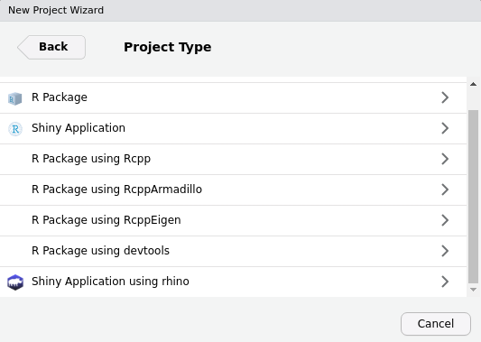
Create an application using the RStudio wizard
If you use RStudio, probably the easiest way to create a new Rhino application is to simply use Create New Project feature. Once Rhino is installed, it will be automatically added as one of the options in RStudio:
Choose it, input the new project name and you are ready to go.
Create an application using rhino::init()
Creating a Rhino application is possible in the R console by running
the init function:
rhino::init("RhinoApplication")There are two things you need to know when choosing this way of initializing your application:
- Rhino will not change your working directory. You need to either open a new R session in your new application directory or manually change the working directory.
setwd("./RhinoApplication")- Rhino relies on options added to the projects
.Rprofilefile. The most robust way to make sure it was correctly sourced is to simply restart the R session.
A result of both paths will be an initial Rhino application with the following structure:
.
├── app
│   ├── js
│   │   └── index.js
│   ├── logic
│   │   └── __init__.R
│   ├── static
│   │   └── favicon.ico
│   ├── styles
│   │   └── main.scss
│   ├── view
│   │   └── __init__.R
│   └── main.R
├── tests
│   ├── cypress
│   │   └── e2e
│   │       └── app.cy.js
│   ├── testthat
│   │   └── test-main.R
│   └── cypress.json
├── app.R
├── RhinoApplication.Rproj
├── dependencies.R
├── renv.lock
└── rhino.yml
If you want to know more about it, check this document.
Running the application
Now, once you are all set up, let’s run it:
shiny::runApp()And here is what you should be seeing right now:
Add your first module
Your application runs, but it doesn’t have any meaningful functionality. Let’s add something there!
Module structure
In Rhino, each application view is intended to live as a Shiny module
and use encapsulation provided by box package.
Rhino already created a good place for new modules, the
app/view directory. Create a file there, named
chart.R:
Calling a module
The next step is to call your new module in your application. First,
you need to import it into your main application file. To do that, add
another box::use section in your app/main.R
file:
# app/main.R
box::use(
app/view/chart,
)
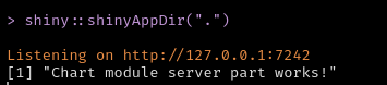
...Now, the main module will be able to use exported functions from
chart.R. Let’s try it! Modify your app/main.R
file to look like that:
# app/main.R

box::use(
  shiny[bootstrapPage, moduleServer, NS],
)
box::use(
  app/view/chart,
)

#' @export
ui <- function(id) {
  ns <- NS(id)

  bootstrapPage(
    chart$ui(ns("chart"))
  )
}

#' @export
server <- function(id) {
  moduleServer(id, function(input, output, session) {
    chart$server("chart")
  })
}
Now, when you run your application, you should see the message from the newly created module:
Adding components to a module
Now is the time to start adding something to your new module. What can we add to a “chart” module? You’re right, a chart. Let’s add a chart with a rhinoceros dataset available in Rhino.
Adding R packages
First, we need to install a library for visualizations - for that, we
will go with echarts4r.
We will be using a total of 5 packages for this application. To save us time in the tutorial we will install them all here.
# In R console
rhino::pkg_install(c("dplyr", "echarts4r", "htmlwidgets", "reactable", "tidyr"))
This function will install the packages, and update
dependencies.R and renv.lock files
accordingly.
Note: Package htmlwidgets is
already installed since it is a dependency for shiny, but
we still should add it to the dependencies.R file.
Add dependencies to the module
Now, once you have both packages available in your project
environment, it’s time to use them. First, you need to import them into
your module. Extend box::use call in your
app/view/chart.R file:
# app/view/chart.R

box::use(
  echarts4r,
  shiny[h3, moduleServer, NS, tagList],
)

...
You can use those packages in your module by calling
{package}${function}. For more options of importing in
box check this link.
Add echarts4r render to the server part of the module
and output part to its UI:
# app/view/chart.R
box::use(
echarts4r,
shiny[h3, moduleServer, NS, tagList],
rhino[rhinos],
)
#' @export
ui <- function(id) {
ns <- NS(id)
tagList(
h3("Chart"),
echarts4r$echarts4rOutput(ns("chart"))
)
}
#' @export
server <- function(id) {
moduleServer(id, function(input, output, session) {
output$chart <- echarts4r$renderEcharts4r(
rhinos |>
echarts4r$group_by(Species) |>
echarts4r$e_chart(x = Year) |>
echarts4r$e_line(Population) |>
echarts4r$e_x_axis(Year) |>
echarts4r$e_tooltip()
)
})
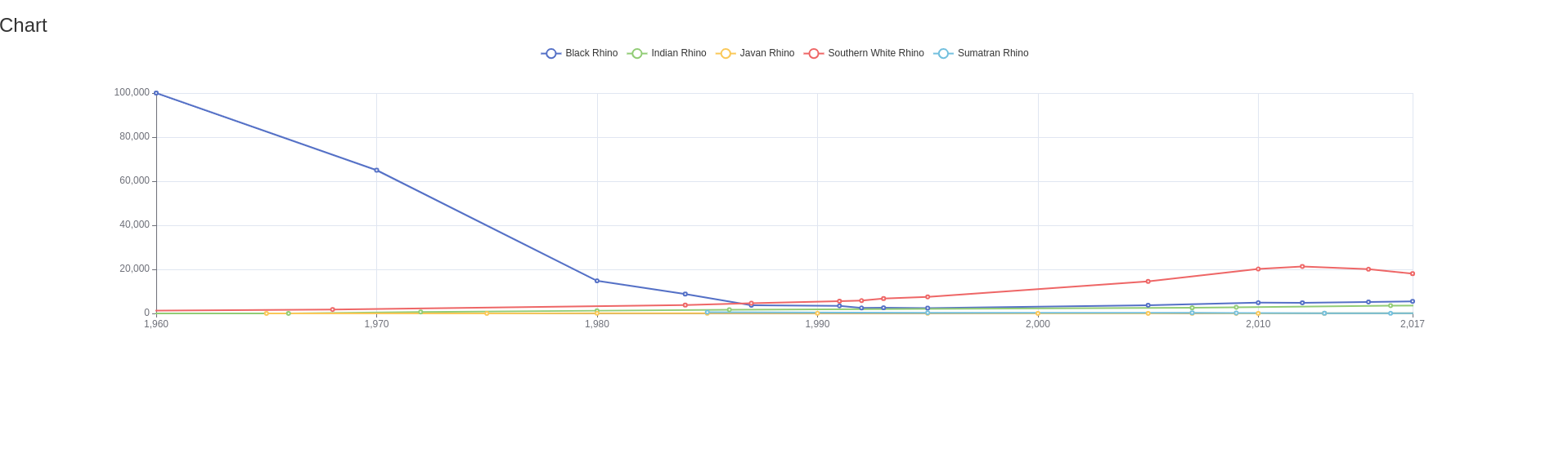
}One thing worth noting here is that in the UI part we had to use
another function from Shiny - tagList. To be able to do
that, you have to adjust your import in box::use - simply
add tagList to the list of imported functions.
Finally, when you run your application, you should see something similar to this:
Add a second module
Once you have some content presented in the application, it would be great to add a table to show the dataset.
For that, let’s create another module -
app/view/table.R:
# app/view/table.R

box::use(
  shiny[h3, moduleServer, NS, tagList],
)

#' @export
ui <- function(id) {
  ns <- NS(id)

  tagList(
    h3("Table")
  )
}

#' @export
server <- function(id) {
  moduleServer(id, function(input, output, session) {

  })
}
Calling the second module
As we did before, we need to call the new module in the
main.R file:
# app/main.R

box::use(
  shiny[bootstrapPage, moduleServer, NS],
)
box::use(
  app/view/chart,
  app/view/table,
)

#' @export
ui <- function(id) {
  ns <- NS(id)

  bootstrapPage(
    table$ui(ns("table")),
    chart$ui(ns("chart"))
  )
}

#' @export
server <- function(id) {
  moduleServer(id, function(input, output, session) {
    table$server("table")
    chart$server("chart")
  })
}
Use the same dataset for both modules
We want to use the same dataset in both modules, so instead of calling it twice, let’s pass data as an argument:
# app/main.R

box::use(
  shiny[bootstrapPage, moduleServer, NS],
  rhino[rhinos],
)
box::use(
  app/view/chart,
  app/view/table,
)

#' @export
ui <- function(id) {
  ns <- NS(id)

  bootstrapPage(
    table$ui(ns("table")),
    chart$ui(ns("chart"))
  )
}

#' @export
server <- function(id) {
  moduleServer(id, function(input, output, session) {
    data <- rhinos

    table$server("table", data = data)
    chart$server("chart", data = data)
  })
}
# app/view/table.R

box::use(
  shiny[h3, moduleServer, NS, tagList],
)

#' @export
ui <- function(id) {
  ns <- NS(id)

  tagList(
    h3("Table")
  )
}

#' @export
server <- function(id, data) {
  moduleServer(id, function(input, output, session) {

  })
}
# app/view/chart.R

box::use(
  echarts4r,
  shiny[h3, moduleServer, NS, tagList],
)

#' @export
ui <- function(id) {
  ns <- NS(id)

  tagList(
    h3("Chart"),
    echarts4r$echarts4rOutput(ns("chart"))
  )
}

#' @export
server <- function(id, data) {
  moduleServer(id, function(input, output, session) {
    output$chart <- echarts4r$renderEcharts4r(
      data |>
        echarts4r$group_by(Species) |>
        echarts4r$e_chart(x = Year) |>
        echarts4r$e_line(Population) |>
        echarts4r$e_x_axis(Year) |>
        echarts4r$e_tooltip()
    )
  })
}
Create a table
For the table, we will go with the reactable
package.
Now you can add a table to the application. Let’s check the raw data for Rhinos:
# app/view/table.R

box::use(
  reactable,
  shiny[h3, moduleServer, NS, tagList],
)

#' @export
ui <- function(id) {
  ns <- NS(id)

  tagList(
    h3("Table"),
    reactable$reactableOutput(ns("table"))
  )
}

#' @export
server <- function(id, data) {
  moduleServer(id, function(input, output, session) {
    output$table <- reactable$renderReactable(
      reactable$reactable(data)
    )
  })
}
The application should look similar to this:
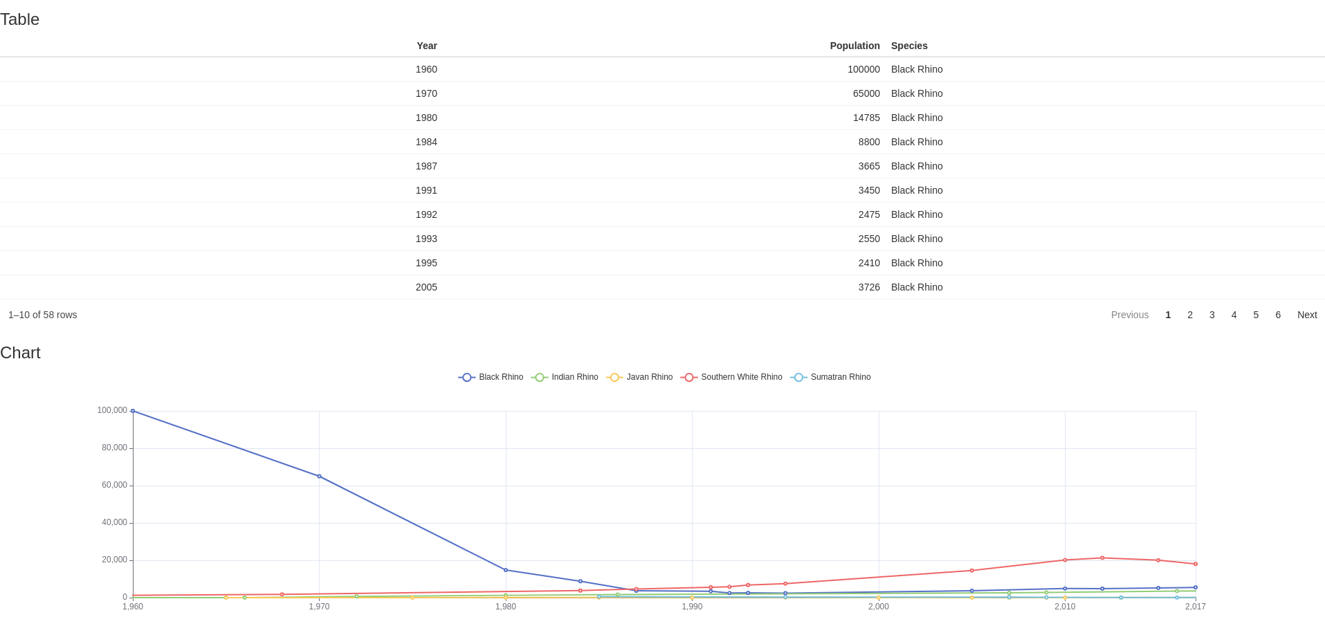
Add logic
It seems that it would be great to slightly adjust the table. Let’s transform the dataset a little bit.
We recommend placing the code which can be expressed without Shiny in
the app/logic directory.
Let’s create a file there, called
app/logic/data_transformation.R.
The table would be better if for each Rhino species we would have a
separate column, so it would be easy to compare populations across time.
To do that, we need to transform the dataset using the
pivot_wider function from the tidyr
package.
Now we are able to access this function in our
data_transformation.R file using box::use().
Let’s also create a function that wraps pivot_wider and
transforms data. Note that, as always, we need to add @export to be able to access it in the file it
is being sourced.
# app/logic/data_transformation.R

box::use(
  tidyr[pivot_wider],
)

#' @export
transform_data <- function(data) {
  pivot_wider(
    data = data,
    names_from = Species,
    values_from = Population
  )
}
The next step is to call this function in your table module.
Add box import and transform dataset:
# app/view/table.R
box::use(
reactable,
shiny[h3, moduleServer, NS, tagList],
)
box::use(
app/logic/data_transformation[transform_data],
)
#' @export
ui <- function(id) {
ns <- NS(id)
tagList(
h3("Table"),
reactable$reactableOutput(ns("table"))
)
}
#' @export
server <- function(id, data) {
moduleServer(id, function(input, output, session) {
output$table <- reactable$renderReactable(
data |>
transform_data() |>
reactable$reactable()
)
})
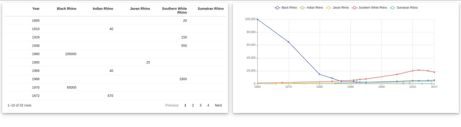
}When you run the application, you should see something similar to this:
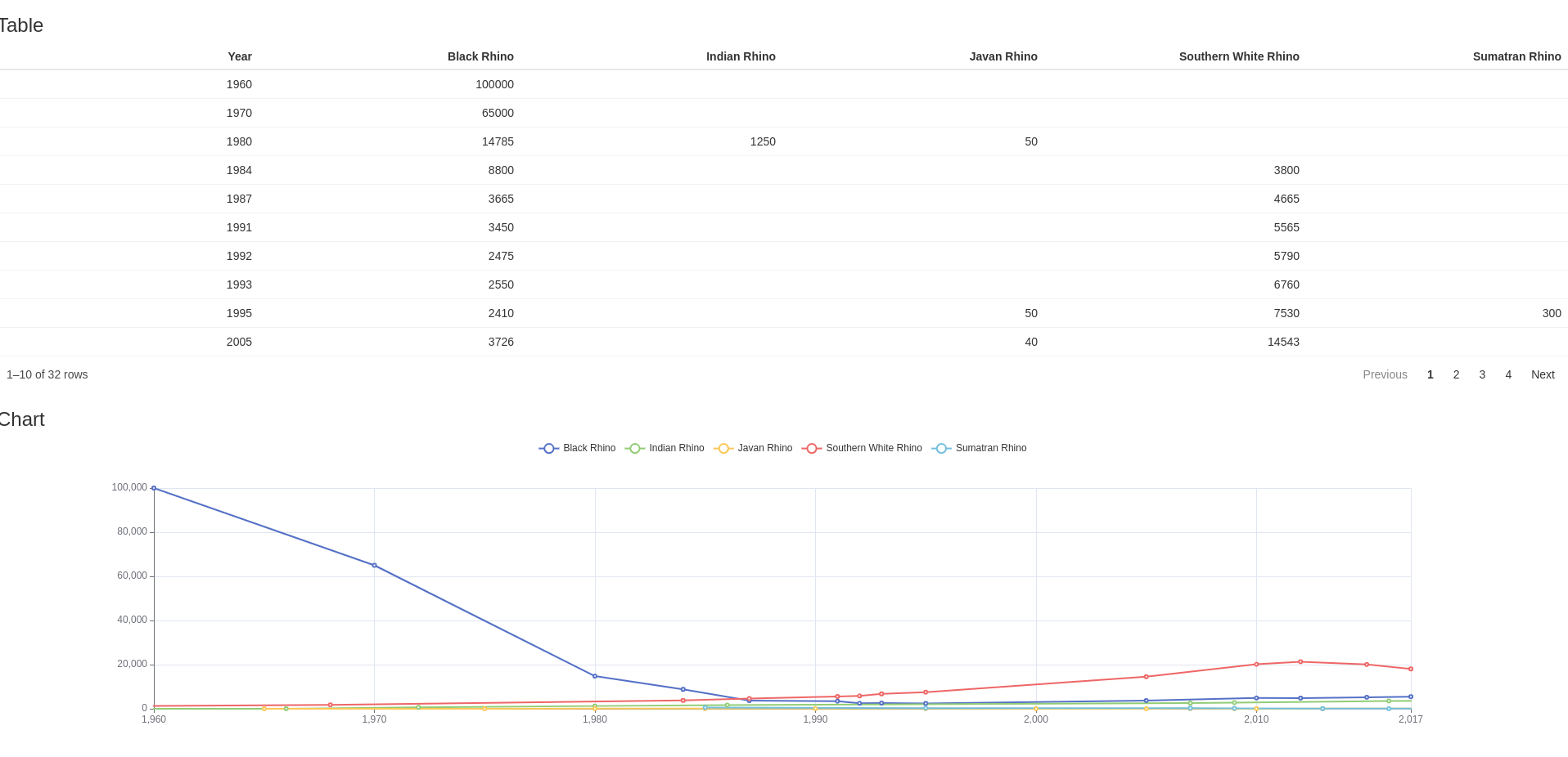
You can notice, that table is arranged by the Black Rhino population.
It would make sense to change it to Year using
dplyr::arrange.
Next, add arrange to transform_data function:
# app/logic/data_transformation.R

box::use(
  dplyr[arrange],
  tidyr[pivot_wider],
)

#' @export
transform_data <- function(data) {
  pivot_wider(
    data = data,
    names_from = Species,
    values_from = Population
  ) |>
    arrange(Year)
}
The result looks much more understandable:
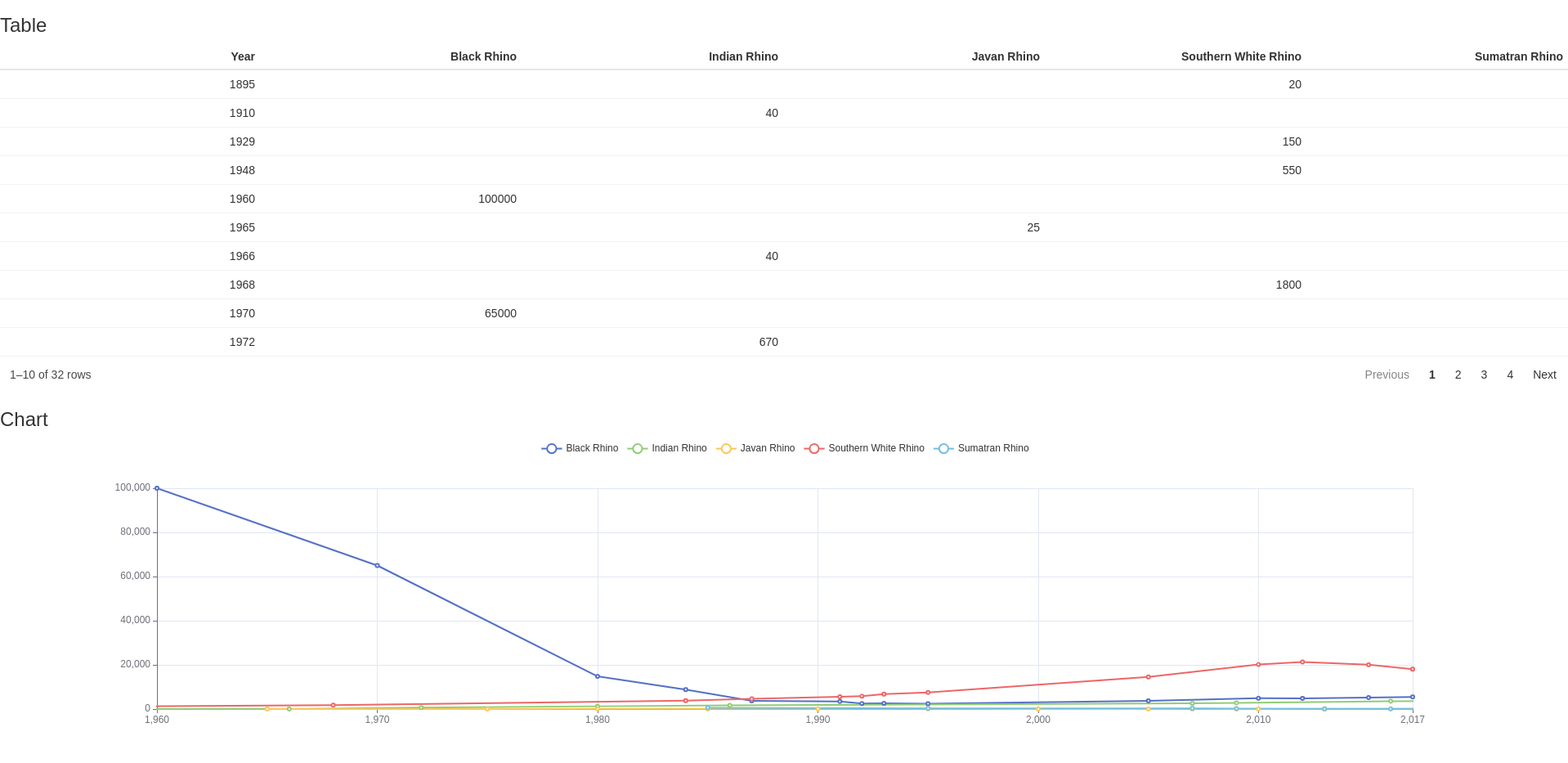
There is still one element that can be improved. If you check the
X-axis in the chart, values contain a comma. It’s the default behavior
for integers, but this is a year! To fix that, you need to add a custom
formatter. Let’s create another file,
app/logic/chart_utils.R:
# app/logic/chart_utils.R

box::use(
  htmlwidgets[JS],
)

#' @export
label_formatter <- JS("(value, index) => value")
Finally, add the formatter to the chart module:
# app/view/chart.R

box::use(
  echarts4r,
  shiny[h3, moduleServer, NS, tagList],
)
box::use(
  app/logic/chart_utils[label_formatter],
)

#' @export
ui <- function(id) {
  ns <- NS(id)

  tagList(
    h3("Chart"),
    echarts4r$echarts4rOutput(ns("chart"))
  )
}

#' @export
server <- function(id, data) {
  moduleServer(id, function(input, output, session) {
    output$chart <- echarts4r$renderEcharts4r(
      data |>
        echarts4r$group_by(Species) |>
        echarts4r$e_chart(x = Year) |>
        echarts4r$e_line(Population) |>
        echarts4r$e_x_axis(
          Year,
          axisLabel = list(
            formatter = label_formatter
          )
        ) |>
        echarts4r$e_tooltip()
    )
  })
}
It should now look better:
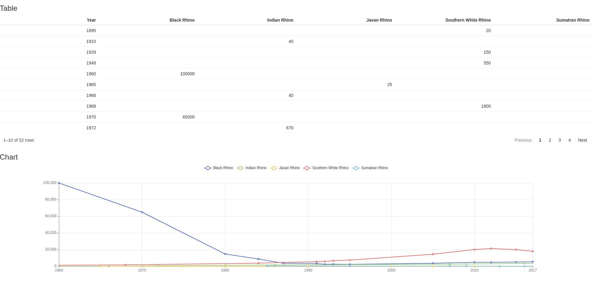
Add custom styles
Note: Sass builder uses Node.js. If you are not
able to install Node in your environment, you can change the
sass entry in the rhino.yml file to
r. It will now use the R package for Sass bundling. Under
the hood, it uses a deprecated C++ library, so the Node solution is
strongly recommended here.
In this stage, the application has working components, but it doesn’t have a clean and organized look to it. For this we will need a little CSS styling.
Adjusting application style can be done by providing custom styles in
the app/styles directory, But first, you need to adjust the
application a little bit by adding HTML tags and CSS classes:
# app/main.R

box::use(
  shiny[bootstrapPage, div, moduleServer, NS],
  rhino[rhinos],
)
box::use(
  app/view/chart,
  app/view/table,
)

#' @export
ui <- function(id) {
  ns <- NS(id)

  bootstrapPage(
    div(
      class = "components-container",
      table$ui(ns("table")),
      chart$ui(ns("chart"))
    )
  )
}

#' @export
server <- function(id) {
  moduleServer(id, function(input, output, session) {
    data <- rhinos

    table$server("table", data = data)
    chart$server("chart", data = data)
  })
}
# app/view/chart.R

box::use(
  echarts4r,
  shiny[div, moduleServer, NS],
)
box::use(
  app/logic/chart_utils[label_formatter],
)

#' @export
ui <- function(id) {
  ns <- NS(id)

  div(
    class = "component-box",
    echarts4r$echarts4rOutput(ns("chart"))
  )
}

#' @export
server <- function(id, data) {
  moduleServer(id, function(input, output, session) {
    output$chart <- echarts4r$renderEcharts4r(
      data |>
        echarts4r$group_by(Species) |>
        echarts4r$e_chart(x = Year) |>
        echarts4r$e_line(Population) |>
        echarts4r$e_x_axis(
          Year,
          axisLabel = list(
            formatter = label_formatter
          )
        ) |>
        echarts4r$e_tooltip()
    )
  })
}
# app/view/table.R

box::use(
  reactable,
  shiny[div, moduleServer, NS],
)
box::use(
  app/logic/data_transformation[transform_data],
)

#' @export
ui <- function(id) {
  ns <- NS(id)

  div(
    class = "component-box",
    reactable$reactableOutput(ns("table"))
  )
}

#' @export
server <- function(id, data) {
  moduleServer(id, function(input, output, session) {
    output$table <- reactable$renderReactable(
      data |>
        transform_data() |>
        reactable$reactable()
    )
  })
}
Now you are ready to modify the styles. Simply add few CSS rules to
app/styles/mains.scss file:
// app/styles/main.scss

.components-container {
  display: inline-grid;
  grid-template-columns: 1fr 1fr;
  width: 100%;

  .component-box {
    padding: 10px;
    margin: 10px;
    box-shadow: 0 4px 8px 0 rgba(0, 0, 0, 0.2), 0 6px 20px 0 rgba(0, 0, 0, 0.19);
  }
}
If you try running the application right now, you will not see any
changes. That is because Rhino uses minified
app/static/app.min.css for styling. To use it, you will
need to build it using the Rhino function:
# in R console
rhino::build_sass()
Now, after running the application you should see something similar to this:
It is worth noting, that you don’t need to add
app/static/app.min.css to your application header - Rhino
does that for you.
Let’s adjust the application a little bit more by adding a title:
# app/main.R

box::use(
  shiny[bootstrapPage, div, h1, moduleServer, NS],
)
box::use(
  app/view/chart,
  app/view/table,
)

#' @export
ui <- function(id) {
  ns <- NS(id)

  bootstrapPage(
    h1("RhinoApplication"),
    div(
      class = "components-container",
      table$ui(ns("table")),
      chart$ui(ns("chart"))
    )
  )
}

...
And some styling:
// app/styles/main.scss

.components-container {
  display: inline-grid;
  grid-template-columns: 1fr 1fr;
  width: 100%;

  .component-box {
    padding: 10px;
    margin: 10px;
    box-shadow: 0 4px 8px 0 rgba(0, 0, 0, 0.2), 0 6px 20px 0 rgba(0, 0, 0, 0.19);
  }
}

h1 {
  text-align: center;
  font-weight: 900;
}
Finally, build Sass once again:
# in R console
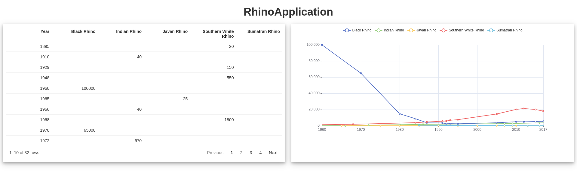
rhino::build_sass()The result should look similar to this:
Add JavaScript code
Note: Rhino tools for JS require Node.js. You
can still use JavaScript code like
in a regular Shiny application, but instead of using
www directory, you should add your files to
static/js and call them using full path,
e.g. tags$script(src = "static/js/app.min.js").
As the last element, let’s add a button that will trigger a JavaScript popup.
First, we need to create a simple button and style it:
# app/main.R

box::use(
  shiny[bootstrapPage, div, h1, icon, moduleServer, NS, tags],
)
box::use(
  app/view/chart,
  app/view/table,
)

#' @export
ui <- function(id) {
  ns <- NS(id)

  bootstrapPage(
    h1("RhinoApplication"),
    div(
      class = "components-container",
      table$ui(ns("table")),
      chart$ui(ns("chart"))
    ),
    tags$button(
      id = "help-button",
      icon("question")
    )
  )
}

...
// app/styles/main.scss
.components-container {
display: inline-grid;
grid-template-columns: 1fr 1fr;
width: 100%;
.component-box {
padding: 10px;
margin: 10px;
box-shadow: 0 4px 8px 0 rgba(0, 0, 0, 0.2), 0 6px 20px 0 rgba(0, 0, 0, 0.19);
}
}
h1 {
text-align: center;
font-weight: 900;
}
#help-button {
position: fixed;
top: 0;
right: 0;
margin: 10px;
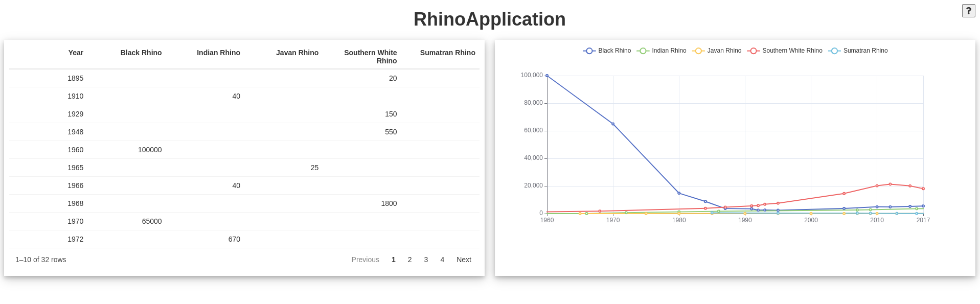
}Remember to rebuild Sass with rhino::build_sass()!
You should now see a button with a question mark in the top right corner of the application:
Now, it’s time for writing the JavaScript code that should show the
popup with a message. All JS code should be stored in the
app/js directory. You already have the first (empty) file
there - index.js. Let’s use it:
// app/js/index.js

export function showHelp() {
  alert('Learn more about Rhino: https://appsilon.github.io/rhino/');
}
This function will simply show a browser alert with the message. If
you are familiar with how JavaScript code is used in Shiny applications,
you will notice one difference - keyword export added
before the function name. In Rhino, only functions marked like that will
be available for Shiny to use.
Same as it was with styles, the Rhino application does not use JS
files directly, but instead utilizes minified version build with
rhino::build_js function. Try it:
# in R console
rhino::build_js()
Now app/static/js/app.min.js file has been created and,
same as the minified CSS file, is automatically included in the
application head tag.
The last thing here is to use the showHelp() function in
the application. To do that, let’s simply add onclick to
the button:
# app/main.R

box::use(
  shiny[bootstrapPage, div, h1, icon, moduleServer, NS, tags],
)
box::use(
  app/view/chart,
  app/view/table,
)

#' @export
ui <- function(id) {
  ns <- NS(id)

  bootstrapPage(
    h1("RhinoApplication"),
    div(
      class = "components-container",
      table$ui(ns("table")),
      chart$ui(ns("chart"))
    ),
    tags$button(
      id = "help-button",
      icon("question"),
      onclick = "App.showHelp()"
    )
  )
}

...
You have probably noticed the second difference between the classic
Shiny approach and the one used in Rhino. All exported JS functions are
now available under App (same as any other JavaScript
function from a library, e.g. Math.round).
Now, if you run the application and click the button, you should see something like this:
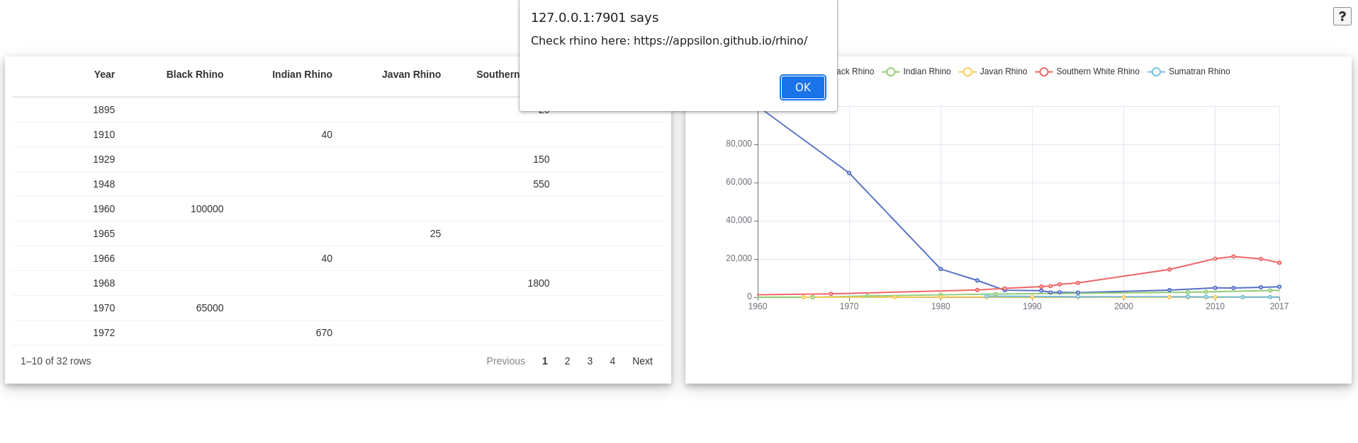
Congratulations! You now have a fully armed and operational
battle station Rhino application!